
How To Measure Black Hole Masses
The Set-up
Most galaxies are home to a central supermassive black hole which is millions to billions times more massive than our sun. For nearby supermassive black holes we can measure the mass by tracking how stars orbit the center of the galaxy and then determine how massive the black hole needs to be to keep everything in place. In order to measure the mass of Sagittarius A*, the black hole in the center of our own Milky Way galaxy, the Keck/UCLA Galactic Center Group have been tracking stars since 1995. Using this data they now know the mass of Sagittarius A* is 4 million times the mass of the sun (see this website for some cool animations). However, we are only able to use this technique for very nearby black holes. Most black holes are too far away for telescopes to be able to image the orbits of these stars.
Reverberation Mapping is a technique which instead uses time delays to measure the radius of clouds orbiting supermassive black holes (developed by some guys named Blandford, McKee, and Peterson). Once the radius and velocity of the clouds are measured it is possible to measure the mass of the black hole. But how exactly does this work?
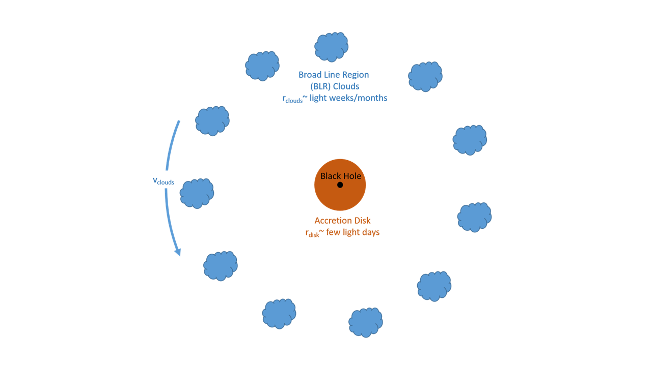
Reverberation Mapping can be used to study Active Galactic Nuclei (AGN). AGN are the highly luminous central regions of galaxies that house a supermassive black hole surrounded by a hot accretion disk which is formed as matter gets pulled into the black hole. We can see the geometry of the system below. The supermassive black hole is in the center of the galaxy and is surrounded by an accretion disk which extends out to a radius of a few light days (1 light day = 26 billion km). Then, further out, there are clouds orbiting at a radius of light weeks to months that form what is known as the Broad Line Region.
Measuring Time Delays
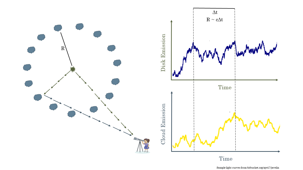
Reverberation mapping takes advantage of the fact the light emitted from AGN is highly variable. There are often flares which are emitted from the accretion disk, near the black hole, as matter is getting pulled in. As shown in the animation below, some of this light goes directly to an observer while some of it gets reflected off the clouds before coming to us. We can measure the time delay between when we first see the flare and when we see the light reflected from the cloud. Now that we know how long it takes for light to get to the clouds and we know how fast light travels (c=3 x 10⁸ m/s) we can determine the radius of the clouds. Remember from your school days that distance traveled = velocity x time.
You may be thinking that sounds too simple. You would be right. Because the light is emitted from around the black hole in all directions you see reflections from the clouds at different times. This is shown in the animation below. What you actually observe is the flare from the black hole and a broad response from the clouds.
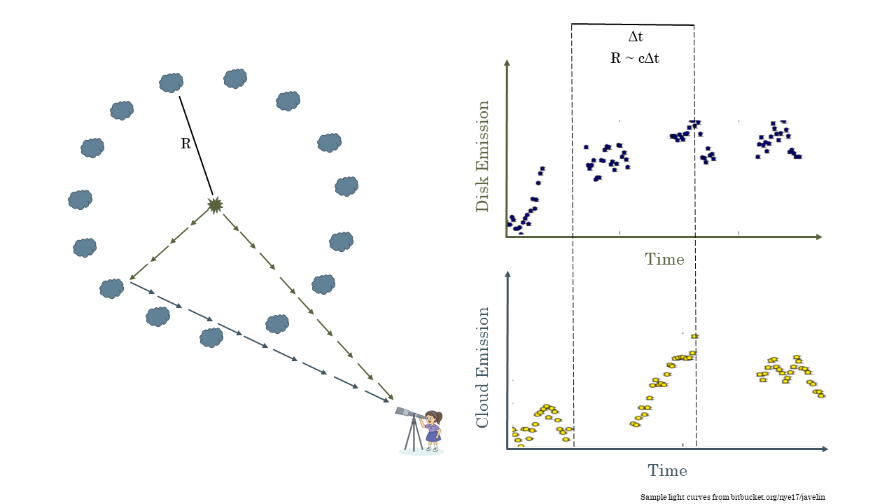
Now you may be asking some more questions: how often do these flares occurs, how long do they last, how does this affect what we observe? These are also excellent questions. These sources are highly variable so you will often observe flares. We can see this in the image below. The disk emission is highly variable but the response from the clouds looks similar but just a bit stretched for the same reason we just talked about. To measure the time lag we measure the delay between peaks in the curves (for the interested mathematically savvy readers we do this using cross correlation functions).
The last complication is due to how long it takes to observe these systems. Some of these black holes are very far away; I observe black holes up to 12 billion light years away. This light had to travel a long time through space which is expanding, which makes the delays appear even longer to us here on Earth. Depending on the black hole and how far away it is these time lags can be months to years long. Given the limited resource of telescope time we have to make due with only observing our black holes every few days to months. This means that what we observe is much more like the picture below. This makes observing time lags difficult but it is still possible. This is what I do as part of the Australian Dark Energy Survey (OzDES) Reverberation Mapping Program. We have been observing the same 771 AGN for 6 years in order to measure the mass of their supermassive black hole.
Measuring Velocities
You have now learned how we calculate the radius the clouds orbiting the black hole but there is still one more piece to the puzzle before we can get the black hole mass. We need to know how fast the clouds are orbiting. When we observe how the clouds respond to the flares we are actually observing how the strength of emission lines which are formed as the clouds are ionized changes. Below we can see a video showing how the response from the clouds changes over four years for one of the AGN we observe with OzDES. We observe this response by looking at the change in strength of emission lines formed when these clouds are ionized. For distant AGN we can observe the C IV emission line. We know that emission lines are always found at the same wavelength. For example, C IV is always emitted at 145.9 nm. However, the Doppler effect says that the wavelength of the emitted light can change if the source emitting the light is moving away from us or towards us. If the light source is moving towards us we say it is blueshifted and the wavelength decreases. If it is moving away from us we say it is redshifted and the wavelength increases. As we see below this leads to a broad line shape. The faster the clouds rotate around the black hole the stronger the red/blueshifting is and the wider the line will be. Therefore we can measure the velocity of the clouds by measuring the width of the emission line.
Measuring Black Hole Mass
Now that we have the radius of the clouds (R) and their orbital velocity (v) we can determine the black hole mass using this simple equation.
M = f R v2/G
This assumes the system is in virial equilibrium (which relates the kinetic energy of a system to its gravitational potential energy). Here G is the gravitational constant (G=6.67x10⁻¹¹ m3kg-1s-2). Now you may be wondering what f represents. What we observe is dependent on other factors we can’t measure for every source – such as the angle at which we observe the AGN. In order to estimate these effects we use the f-factor, a unitless number measured to be around 5. It is calculated by looking at AGN that are close enough for us to measure the mass using both reverberation mapping and by measuring the orbits of stars around the black hole. The factor which brings these two measurements into agreement is averaged for many AGN and that gives us the f-factor.
I have published the first two black hole mass measurements made by OzDES in this paper here. They have masses over a billion times more massive than our sun. This is just the tip of the iceberg and we will have many more black hole mass measurements ready to be published soon!