Calibrating Spectra with OzDES_calibSpec
OzDES_calibSpec is a publically available code which can be found at github.com/jhoormann/OzDES_calibSpec. This methodlogy was first presented in the paper CIV Black Hole Mass Measurements with the Australian Dark Energy Survey (OZDES) by Hoormann et al 2019.
Reverberation mapping (RM) works by measuring variations in the size of emission lines in order to measure the response from the clouds (go to this blog to learn more about how RM works). In the video below you can see how this works. This video show the C IV emission line as observed by OzDES for the active galaxy DES J0033-42 as it changes over time. You can see that the emission line changes in size which translates to a change in flux in the light curve shown in the panel on the top right.
 The change in line strength corresponds to flares which occur right around the black hole. However, there are other factors which could cause variations to appear which have nothing to do with underlying physics of black holes.
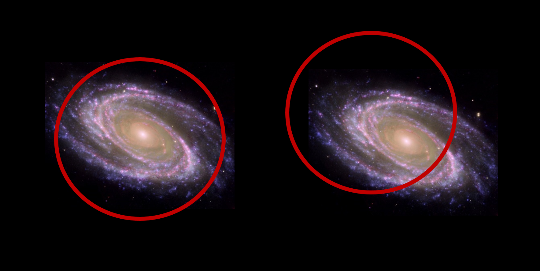
A number of things could happen to affect the shape of the spectrum we observe. Something as simple as a wispy cloud floating above the telescope while we are observing could block some of the light and make the source appear dimmer. Also, because of the orbit of the earth, even though we are looking at the same patch of the universe over and over again, the fields we target will appear in different parts of the sky based on the time of year we observe them. If we observe something just above the horizon the light will have to travel through more atmosphere than if we observe it when it is directly overhead. This can also cause changes in what we observe. Another effect is due to the experimental set-up. OzDES uses a system called 2dF which allows you to place optical fibers exactly where you expect the source you want to observe to be. Ideally the optical fiber is positioned at the center of the galaxy in order to collect all the light that it emits. This is shown in the left panel of the image below. However, it is possible for the fiber to be offset (right) meaning that we will be unable to collect light from parts of the galaxy.
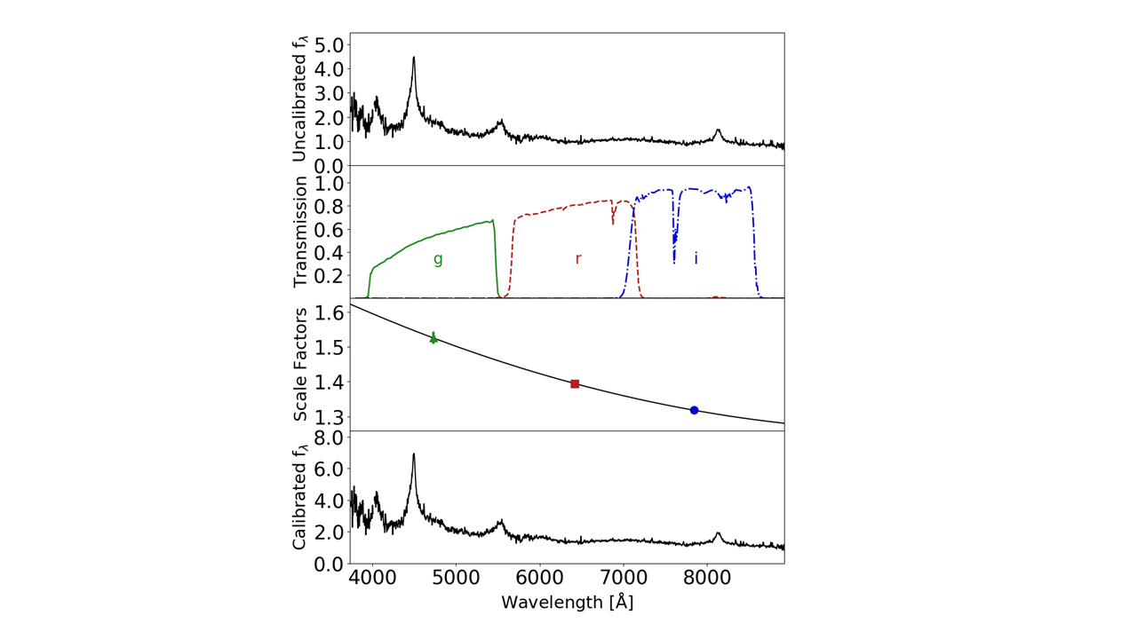
One of the primary projects I have led is to determine how best to account for all of these variations so that we can perform high quality calibration of our spectra. The way I do this is using a procedure called spectrophotometric calibration. This means that we use high quality calibrated photometry (in our case using the near simultaneous DES observations) to calibrate our spectra. How this works is illustrated in the figure below. In the top panel is an example of an uncalibrated spectrum that we have observed with OzDES. In order to compare a spectrum to photometry you need to convert your spectrum into magnitudes. Because we will be comparing our calculated OzDES magnitudes to the data observed by DES we use their transmission functions (second panel). The transmission functions tell us, for each band DES observes (we care about the g, r, i bands because that is what overlaps with our OzDES spectrum) what percentage of the light at a given wavelength will be observed by DES. I can then compare the calculated OzDES magnitudes with the magnitudes observed at the same time by DES and calculate the scale factor needed to bring the two values into agreement. The third panel shows these scale factors. The error bars on these values are so small in large part due to the fact that the DES photometry we are using is so precise (sub percent accuracy). As you can see the scale factors are not constant. Therefore, I fit a 2D polynomial to the scale factors to create a scaling function which I multiply by the original spectrum to calibrate it. The uncertainty in this scaling function is estimated using Gaussian processes and is then added in quadrature with the uncertainties due to the observations themselves.
The fact that the scale factors are not constant for each band is likely due to a combination of all of the effects that were mentioned above. Even between observations of the same source the scaling function can change significantly. That is why having near simultaneous photometric observations are so important, at least if you are calibrating a variable source such as the active galaxies observed for the RM program.
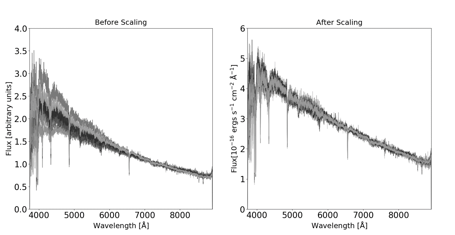
In order to test how well this calibration procedure works I made use of the fact that every time OzDES observes it targets what are called F-stars. These F-stars are non-varying stars with a well understood spectral shape which makes them ideal targets for calibration purposes. In the figure below are all of the observations through OzDES Year 4 for the F-star FSC0225m0444. In the left panel you can see the original, uncalibrated spectra. Despite the fact that this star should have a constant spectral shape you can see that data does vary, particularly at lower wavelengths. However, after calibration (right panel) you can see that all the observations do indeed yield similar spectra.
In order to quantify how well this procedure works I took the calibrated F-star spectrum and calculated the root mean squared (RMS) spectrum. The calibrated F-star spectrum is shown again in the top panel of the next figure and the RMS spectrum is shown in the middle panel. The RMS spectrum isolates the variation in the input data. I can then calculate the fractional variation for this source. This is shown as the percent variation in the bottom panel of the plot below.
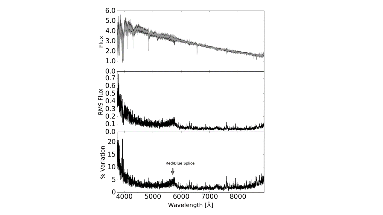
The percent variation is generally less than 5%. The variation is larger at lower wavelengths where the observations themselves are nosier. There is also an increase in variation around 5700 Angstroms. This is because the spectrograph OzDES uses (AAOmega) breaks up the data into two arms, the red (high wavelength) and blue (low wavelength) arms. The break between the arms occurs at 5700 Angstroms. In order to get a single spectrum the data from the two arms are spliced together. While the procedures to do this have gotten better and better over the years there is still some added uncertainty where the splicing happens. The fact that on the whole the uncertainty is less than 5% though is fantastic! This puts us at the threshold of the noise levels of the detectors themselves!
While this code, OzDES_calibSpec, was designed with the OzDES Reverberation Program in mind it can be applied to any spectrum with corresponding photometry data.